Abstract. In computer-vision generation tasks, diffusion models have demonstrated remarkable performance, and flow matching improves inference efficiency by replacing an SDE with an ODE. As the first open-source 7B-scale diffusion language model (DLM), LLaDA shows strong promise, suggesting that diffusion language models may eventually replace the widely used autoregressive paradigm. This raises a natural question: can models guided by discrete flow matching achieve better performance? However, our theoretical analysis indicates that the current diffusion language model LLaDA is, in fact, already equivalent to a discrete flow matching model.
1. Introduction
(Omitting some related works…)
Here, I will explain why LLaDA is a Discrete Flow Matching model. At a conceptual level, continuous flow matching can be viewed as addressing the fact that the randomness in continuous diffusion models often makes generation require many iterative steps. In diffusion language models, especially LLaDA, each token typically moves directly from [MASK] to a concrete token (ignoring the remasking mechanism), so this “stochasticity” issue is much less pronounced, and discrete diffusion and discrete flow matching become effectively equivalent. More concretely, since the “velocity” is defined as a probability-flow velocity, the model is trained to predict an accurate posterior distribution; LLaDA is also learning to predict this posterior. When the loss is chosen as cross-entropy, the resulting objective matches LLaDA exactly.
This note reviews (i) denoising diffusion probabilistic models (DDPMs) [1] in continuous spaces as stochastic forward–reverse processes and (ii) flow matching [2] as a deterministic alternative based on ordinary differential equations. We then summarize discrete diffusion (e.g., D3PM [3]) and discrete flow matching [4], [5], and explain why the LLaDA training objective [6] can be interpreted as a discrete flow matching objective.
2. Preliminaries
Unless otherwise specified, throughout the rest of this note, subscript 0 denotes clean data and subscript 1 denotes noise.
2.1 Diffusion models and flow matching in continuous spaces
Denoising diffusion probabilistic models (DDPMs) [1] were originally developed and widely used in continuous domains. They define a noise-injection forward process and a learned reverse denoising process.
Forward (noising) process. Let \(x_0\) denote data and \(x_{1:T}\) denote a sequence of latent variables. A standard Gaussian forward process is
\[q(x_{1:T} \mid x_0) = \prod_{t=1}^{T} q(x_t \mid x_{t-1}), \tag{1}\] \[q(x_t \mid x_{t-1}) = \mathcal{N}\big(x_t;\ \sqrt{\alpha_t}\, x_{t-1},\ (1-\alpha_t) I\big), \tag{2}\] \[\text{equivalently}\quad x_t = \sqrt{\bar\alpha_t}\, x_0 + \sqrt{1-\bar\alpha_t}\,\epsilon, \qquad \epsilon \sim \mathcal{N}(0, I), \tag{3}\]where \(\bar\alpha_t := \prod_{s=1}^{t} \alpha_s\).
Reverse (denoising) process. The learned reverse dynamics are typically parameterized as
\[p_\theta(x_{t-1} \mid x_t) = \mathcal{N}\big(x_{t-1};\ \mu_\theta(x_t, t),\ \Sigma_\theta(x_t, t)\big), \tag{4}\] \[p_\theta(x_0, x_1, \ldots, x_T) := p(x_T) \prod_{t=1}^{T} p_\theta(x_{t-1} \mid x_t). \tag{5}\]Because diffusion sampling can be viewed as solving an SDE and injects random noise at each step, many steps are often required for high-quality samples.
Flow matching. To accelerate sampling, flow matching replaces the stochastic SDE with a deterministic ODE [2]. One defines a velocity field \(\mathbf{v}(x_t, t)\) and evolves samples according to
\[\frac{dx_t}{dt} = \mathbf{v}(x_t, t). \tag{6}\]A common construction specifies a probability path via linear interpolation of endpoint distributions,
\[p_t(x) = (1-t)\, p_T(x) + t\, p_0(x), \qquad t \in [0, 1]. \tag{7}\]Flow matching then trains a model \(\mathbf{v}_\theta(x, t)\) to approximate the target velocity field \(\mathbf{v}(x, t)\) along the path.
2.2 Discrete diffusion and discrete flow matching
To transfer the generative capabilities of diffusion and flow matching to discrete domains, researchers have developed discrete diffusion models and discrete flow matching methods.
Discrete diffusion (D3PM). In discrete spaces, Gaussian noise is not directly applicable. D3PM instead defines the forward process through Markov transition matrices \(\{\mathbf{Q}_t\}_{t=1}^{T}\) [3]:
\[[\mathbf{Q}_t]_{ij} = q(x_t = j \mid x_{t-1} = i), \tag{8}\] \[q(\mathbf{x}_t \mid \mathbf{x}_{t-1}) = \mathrm{Cat}\big(\mathbf{x}_t;\ \mathbf{p} = \mathbf{x}_{t-1}\mathbf{Q}_t\big), \tag{9}\] \[q(\mathbf{x}_t \mid \mathbf{x}_0) = \mathrm{Cat}\big(\mathbf{x}_t;\ \mathbf{p} = \mathbf{x}_0 \bar{\mathbf{Q}}_t\big), \qquad \bar{\mathbf{Q}}_t := \mathbf{Q}_1 \mathbf{Q}_2 \cdots \mathbf{Q}_t. \tag{10}\]A widely used choice is absorbing-state diffusion, where noise corresponds to replacing tokens by a [MASK] symbol:
Discrete flow matching. A direct velocity in token space is ill-defined due to discrete jumps. Discrete flow matching therefore defines a probability-space transition rate (an “ODE” in distribution space) [4], [5]. For the \(i\)-th token, a typical form is
\[\nu_t^i(x^i, x_t) = \frac{\dot\kappa_t}{1-\kappa_t}\Big[p_{0 \mid t}(x^i \mid x_t) - \delta_{x_t}(x^i)\Big], \tag{12}\]where \(\nu_t^i \in \mathbb{R}^{\lvert \mathcal{V} \rvert}\) is a probability transition-rate tensor indicating how quickly the \(i\)-th token transitions to other vocabulary elements. Equivalently,
\[\nu_t^i(x, x_t) = \underbrace{\frac{\dot\kappa_t}{1-\kappa_t}}_{\text{time coefficient}} \Big[\, \underbrace{p_{0 \mid t}(x \mid x_t)}_{\text{inflow (destination)}} - \underbrace{\delta_{x_t}(x)}_{\text{outflow (source)}} \,\Big]. \tag{13}\]After evolving the categorical distribution for a small time step \(h\), one samples the next token:
\[X_{t+h}^i \sim \mathrm{Categorical}\Big(\delta_{X_t^i}(\cdot) + h\, \nu_t^i(\cdot, X_t)\Big). \tag{14}\]Therefore, we train the model to output \(p_\theta(x \mid x_t)\) to predict \(p_{0 \mid t}(x \mid x_t)\), so that we can get the velocity.
3. Why LLaDA can be viewed as a flow matching model
We compare continuous flow matching (CFM) and discrete flow matching (DFM).
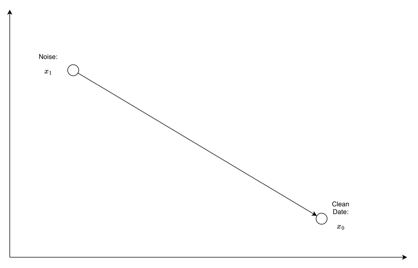
CFM intuition. In CFM, in training time, one may view the instantaneous velocity as the average velocity over the full path from noise to data. For example, under a linear interpolation \(x_t = (1-t)\,x_1 + t\,x_0\), the velocity is constant and equals \(v_t = x_0 - x_1\) as the ground-truth.
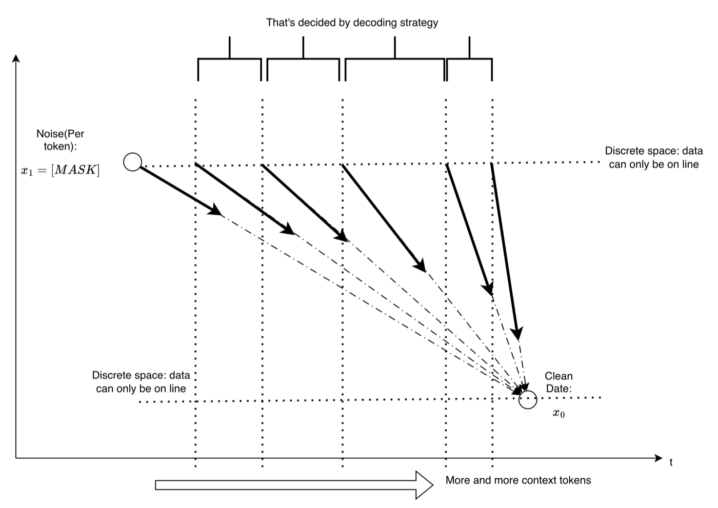
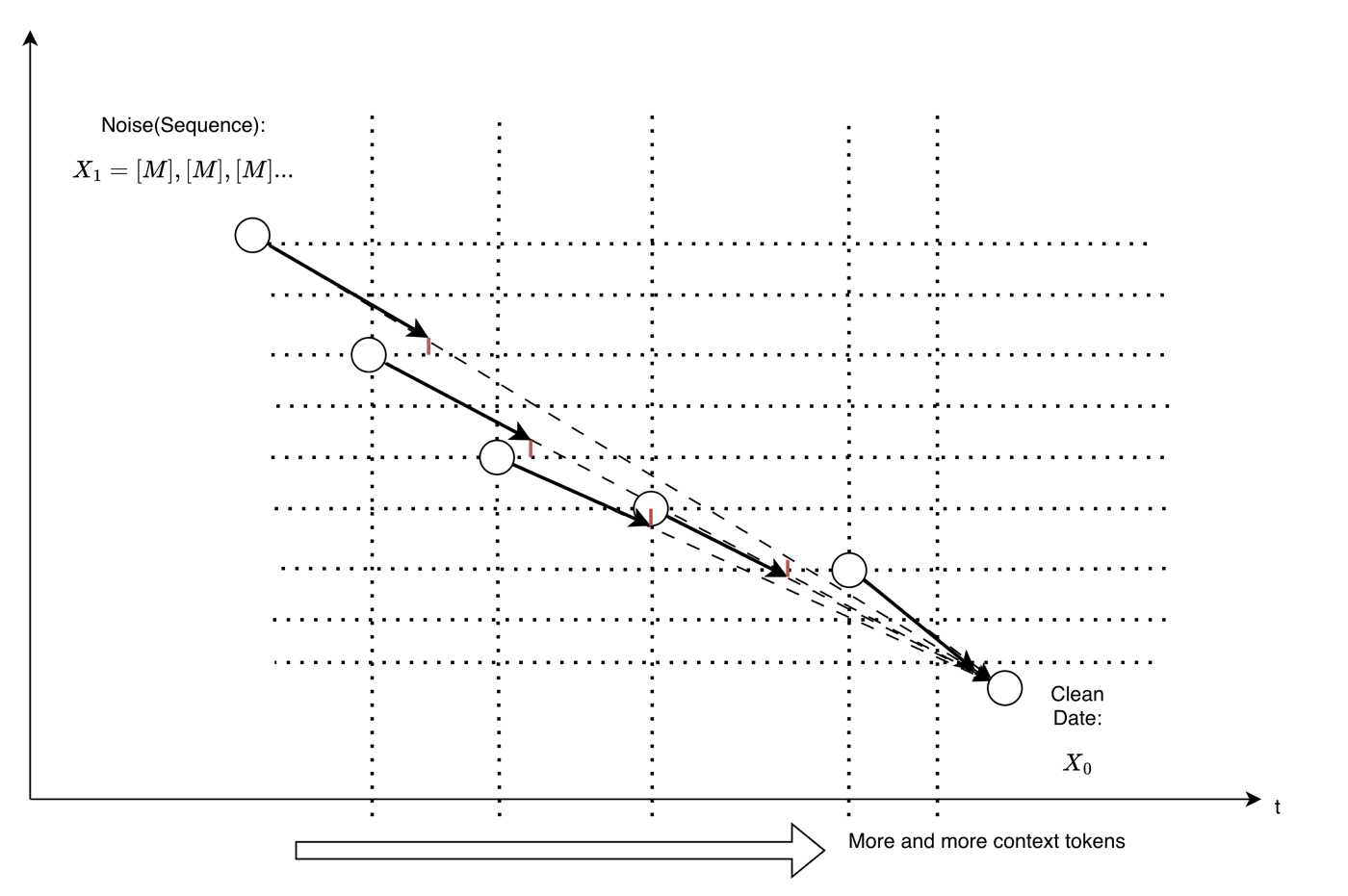
[MASK] and the ground-truth token; as more context is decoded during training, the velocity (shown as the slope) increases, so after multiplying by the same coefficient \(h\), the probability mass transferred toward the ground truth becomes larger, eventually making the sampled token correct. Right: sequence-wise trajectory, where each horizontal dashed line represents a decoding state; because sampling forces the sequence back onto these lines, the red short vertical segments appear as offsets, making the induced flow discontinuous.DFM intuition. In DFM, the instantaneous velocity at time \(t\) is better interpreted as the average velocity over the remaining process from the current partially noised state to the ground truth. For each token, the transition rate is
\[\nu_\tau^i(x, X_\tau) = \frac{\dot\kappa_\tau}{1-\kappa_\tau}\Big[p_{0 \mid \tau}(x \mid X_\tau) - \delta_{X_\tau}(x)\Big], \tag{15}\]where \(x\) can be any token ranging over the vocabulary. Here \(X_1\) is a fully masked sequence (all tokens are [MASK]) with the same length as \(X_0\), and \(p_{0 \mid \tau}(x \mid X_\tau)\) is the posterior distribution over clean tokens given a partially masked sequence.
Using the full-path average transition rate at \(\tau = 1\) is undesirable because all training examples share the same start point (a fully masked \(X_1\)), which makes the learning signal ambiguous and can hinder convergence.
More fundamentally, because discrete sampling alternates between (i) evolving a distribution in probability space and (ii) resampling a discrete token, the induced trajectory is not a single straight line in probability space but a sequence of segments whose behavior depends on the current context. Consequently, using a full-path average as a ground-truth instantaneous rate can introduce systematic bias due to the repeated resampling offsets. This motivates using the remaining-path average velocity as the instantaneous target.
Loss reduction (constant \(\kappa\) simplification). For exposition, suppose \(\kappa\) is constant so the time coefficient can be absorbed. Then the model predicts
\[\nu_{\theta,\tau}^i(x, X_\tau) = p_\theta(x \mid X_\tau) - \delta_{X_\tau^i}(x), \tag{16}\]and we match it to the target
\[\bar\nu_\tau^i(x, X_\tau) = p_{0 \mid \tau}(x \mid X_\tau) - \delta_{X_\tau^i}(x). \tag{17}\]Thus a generic rate-matching loss becomes
\[\begin{aligned} \ell_\theta(\tau, X_\tau) &= \mathrm{LOSS}\Big(\nu_{\theta,\tau}^i(x, X_\tau) - \bar\nu_\tau^i(x, X_\tau)\Big) \\ &= \mathrm{LOSS}\Big(\big[p_\theta(x \mid X_\tau) - \delta_{X_\tau^i}(x)\big] - \big[p_{0 \mid \tau}(x \mid X_\tau) - \delta_{X_\tau^i}(x)\big]\Big) \\ &= \mathrm{LOSS}\Big(p_\theta(x \mid X_\tau),\ p_{0 \mid \tau}(x \mid X_\tau)\Big). \end{aligned} \tag{18–20}\]When LOSS is instantiated as cross-entropy, this yields the LLaDA objective. In this sense, LLaDA can be interpreted as learning the remaining-path average transition rate, i.e., a discrete flow matching model.
References
- Jonathan Ho, Ajay Jain, and Pieter Abbeel. Denoising diffusion probabilistic models. In Advances in Neural Information Processing Systems (NeurIPS), volume 33, pages 6840–6851, 2020.
- Yaron Lipman, Ricky T. Q. Chen, Heli Ben-Hamu, Maximilian Nickel, and Matt Le. Flow matching for generative modeling. In International Conference on Learning Representations (ICLR), 2023.
- Jacob Austin, Daniel D. Johnson, Jonathan Ho, Daniel Tarlow, and Rianne van den Berg. Structured denoising diffusion models in discrete state-spaces. In Advances in Neural Information Processing Systems (NeurIPS), volume 34, pages 17981–17993, 2021.
- Itai Gat, Tal Remez, Neta Shaul, Felix Kreuk, Ricky T. Q. Chen, Gabriel Synnaeve, Yossi Adi, and Yaron Lipman. Discrete flow matching. In Advances in Neural Information Processing Systems (NeurIPS), 2024.
- Andrew Campbell, Jason Yim, Regina Barzilay, Tom Rainforth, and Tommi Jaakkola. Generative flows on discrete state-spaces: Enabling multimodal flows with applications to protein co-design. In International Conference on Machine Learning (ICML), 2024.
- Shen Nie, Fengqi Zhu, Zebin You, Xiaolu Zhang, Jingyang Ou, Jun Hu, Jun Zhou, Yankai Lin, Ji-Rong Wen, and Chongxuan Li. Large language diffusion models. arXiv preprint arXiv:2502.09992, 2025.